Why One Formula Can't Forecast Every SKU
Key takeaway: Many inventory tools apply a single weighted moving average to every SKU. That formula fails seasonal products (misses the ramp), intermittent products (overreacts to zeros), and trending products (lags behind). Different demand patterns need different statistical models.
An illustrative scenario, not a real account.
Say a SKU sells 800 units in October, 1,200 in November, 2,400 in December, then 300 in January. Every year. Same pattern. You could set your calendar by it.
Your inventory tool uses a weighted moving average. It watches October's 800 and suggests a reorder based on roughly that run rate. By the time November's 1,200 pulls the average up, the supplier needs 30 days to ship. December's spike arrives. Your inventory does not.
The tool was not broken. The math worked exactly as designed. The problem was that one formula cannot handle a product that triples in demand over eight weeks and then crashes back down. A weighted moving average was never built for that.
The Dirty Secret of Many Inventory Forecasting Tools
Here is what many mid-market inventory tools do under the hood: they take your recent sales, weight the newer data a little heavier than the older data, and project forward. That is a weighted moving average. It goes by different names in different products ("demand velocity," "sales-weighted forecast," "adaptive averaging"), but the math is the same.
It works fine for a certain type of product. The type that sells roughly the same amount every day, week after week, with minor fluctuations. Toilet paper. Phone cases. Basic supplements.
The problem is that your catalog is not made entirely of phone cases.
Four Patterns, One Formula
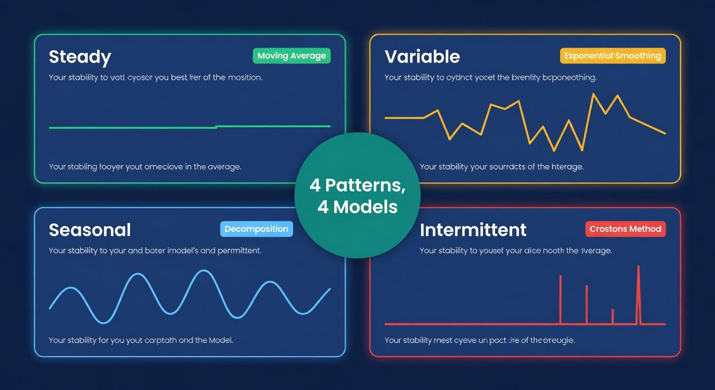
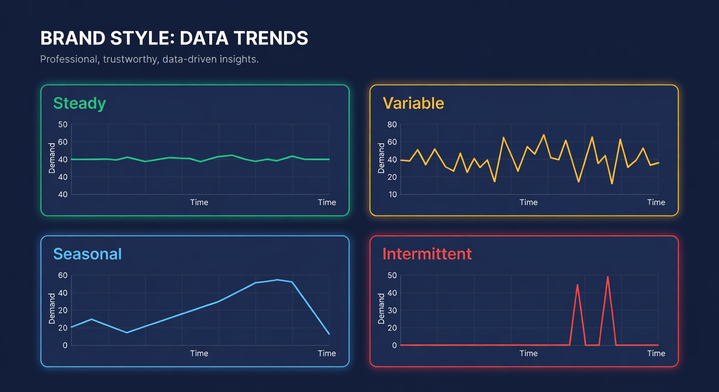
Most SKUs fit one of these demand patterns, and a mixed catalog can easily have all four.
Steady demand
Consistent daily sales with small random fluctuations. A product sells 40-50 units per day, every day, month after month. Forecasting this is easy. A weighted moving average handles it well because tomorrow looks like yesterday.
Variable demand
Unpredictable volume swings with no repeating pattern. A product sells 20 units one day, 80 the next, 10 the day after. No seasonality, no trend. Just chaos. Variable demand is common in categories driven by viral content, ad spend changes, or competitor stock levels.
Seasonal demand
Predictable, recurring time-based patterns. The October-to-December ramp described above. Pool supplies in spring. Tax software in March. The demand shape repeats, but a rolling average cannot see the shape. It only sees the numbers directly behind it.
Intermittent demand
Long gaps between sales, then sudden bursts. A replacement part that sells zero units for three weeks, then 50 in a day when a distributor places a batch order. Intermittent demand is hard to forecast, and a single average handles it badly.
How One Formula Fails Each Type
| Demand Pattern | What the weighted average does | What actually happens | The cost |
|---|---|---|---|
| Steady | Works well | Minor forecast errors | Minimal: this is the easy case |
| Variable | Chases yesterday's number | Overorders after spikes, underorders after dips | Chronic stock imbalance, excess on swing SKUs |
| Seasonal | Catches the ramp late, catches the crash late | Orders arrive after the peak, surplus sits through the off-season | Missed sales during ramp + storage costs on the tail |
| Intermittent | Averages in the zeros | Treats a 50-unit burst product as a 2-unit-per-day product | Perpetual stockouts on slow-but-important SKUs |
That table is the whole argument. If your forecast engine applies the same weighted average across all four types, three of the four are getting the wrong math.
The seasonal failure gets expensive fast
Here are the numbers, because this is where the money disappears.
Say you have a seasonal product with a 30-day supplier lead time. True demand follows this pattern:
| Month | Actual monthly demand |
|---|---|
| Sep | 600 |
| Oct | 900 |
| Nov | 1,800 |
| Dec | 3,000 |
| Jan | 400 |
Illustrative numbers, not real data.
A 3-month weighted average sitting in September sees the average of Jul/Aug/Sep: maybe 550 units per month. It suggests you order for 550. You need 1,800 for November, but your order is already placed based on 550. By the time October's 900 pulls the average to maybe 700, you are placing your November delivery order. You need 3,000 for December.
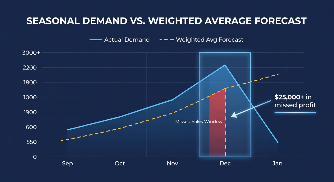
You are always one season behind. The average is a rearview mirror, and seasonal products need a windshield.
At a $25 unit margin, understocking December by even 1,000 units is $25,000 in missed profit. From one SKU.
The intermittent failure is the most misunderstood
A product that sells 0, 0, 0, 0, 50, 0, 0, 0, 0, 0, 60, 0, 0, 0, 0 units per day has an average daily demand of about 7.3 units. A weighted moving average produces something close to that number and suggests you keep 7-8 days of supply on hand.
But the product does not sell 7 units per day. It sells nothing for weeks and then sells 50 at once. Keeping 56 units on hand (8 days at 7/day) means you are fine for a burst of 50, but only if the burst happens in the first week. If it happens after two weeks of zeros, the system may have already flagged the product as overstocked and told you to stop reordering.
Standard formulas cannot separate the "how much" from the "how often" in intermittent demand. They mash both into a single average and lose the signal.
The Right Approach: Match the Model to the Pattern
This is not a new idea. Statisticians figured this out decades ago. Different demand patterns need different statistical models.
For steady demand: Exponential smoothing (ETS) works well. It is a cousin of the weighted moving average but with a tunable smoothing parameter that adapts to the signal-to-noise ratio. Textbook stuff. Published by Holt in 1957.
For seasonal demand: The Holt-Winters extension of exponential smoothing adds a seasonal component. It learns the seasonal shape from prior years and applies it forward. When it sees September, it already knows December is coming. This method has been in supply chain textbooks since the 1960s.
For intermittent demand: Croston's method, published in 1972, splits the problem in two. It separately estimates the average demand size (when a sale happens) and the average interval between demands. This avoids the zeros-dragging-down-the-average problem entirely.
For variable demand: This is where it gets harder. Variable demand with no pattern is genuinely difficult to forecast. The best approach is usually a conservative model with wider safety stock bands, accepting that you cannot predict the noise and protecting against it with buffer instead.
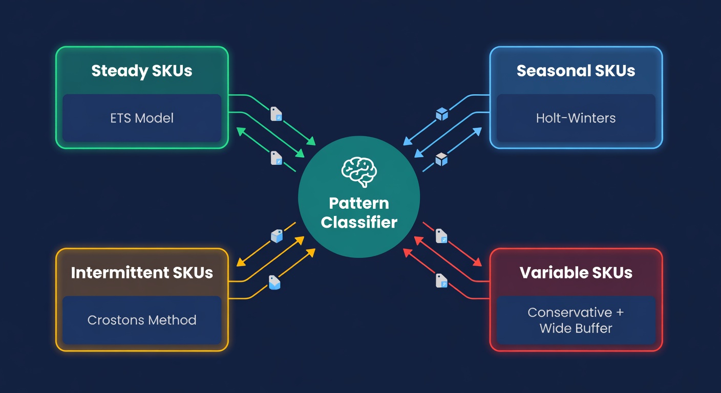
The models exist. They are published. They are well understood. The question is whether your forecasting tool actually uses them, or whether it runs the same weighted average on everything and calls it "AI-powered forecasting."
The Classification Problem
Knowing that different models exist is step one. Step two is figuring out which model applies to which SKU.
You are not going to do this manually. If you have 500 SKUs, you are not going to plot each one's demand history, eyeball the pattern, and assign a model. And even if you did, products change. A steady seller picks up a seasonal pattern when it gets featured in a gift guide. An intermittent product starts selling consistently after a viral TikTok. The classification has to be automatic and it has to update.
We are not going to publish exactly how ReplenishRadar does this. The detection and selection logic is our proprietary engine, and a blog post is no place to hand it to competitors. What we can say is that we analyze each SKU's demand history, classify its pattern, and route it to the appropriate statistical model. Automatically. Continuously. When a product's demand pattern shifts, the model assignment shifts with it.
That is the part many inventory tools skip. Not because the math is impossible: the academic methods have been around for 50+ years. But because building a system that classifies thousands of SKUs and routes each one correctly is hard engineering work. It is much easier to run a single weighted average on everything and call it a day.
How to Tell If Your Tool Does This
Here is a quick test. Go into your inventory tool and look at any SKU's forecast. Ask these questions:
-
Is there any mention of demand type or pattern? If the tool shows a forecast number but never tells you whether the SKU is seasonal, intermittent, or steady, it probably is not differentiating.
-
Does a seasonal product's forecast anticipate the ramp? Look at a product you know has seasonal demand. Does the forecast for three months out reflect the seasonal peak, or does it just project the current run rate forward?
-
Does an intermittent product's reorder point make sense? Find a slow-moving product that sells in bursts. Is the reorder point based on the burst size, or on the averaged-down daily demand?
If all three answers are no, you are running one formula across your entire catalog. That means your seasonal SKUs are systematically understocked during peaks and overstocked during valleys. Your intermittent SKUs are chronically understocked because the zeros kill the average. And you are leaving money on the table in both directions.
The Dollar Impact Across a Whole Catalog
Here is what single-formula forecasting can cost on a hypothetical 500-SKU catalog.
| SKU segment | % of catalog | Avg forecast error (single formula) | Avg forecast error (matched models) | Revenue at risk per month |
|---|---|---|---|---|
| Steady | 45% | 12% | 10% | Low: minimal difference |
| Variable | 20% | 35% | 28% | $18,000 in overstock carrying cost |
| Seasonal (during ramp) | 15% | 55% | 18% | $42,000 in missed sales |
| Intermittent | 20% | 60% | 25% | $11,000 in stockouts |
| Total | $71,000/month |
Illustrative numbers, not real data.
The steady sellers are fine either way. They always were. The gap shows up in the other 55% of the catalog, the SKUs where a weighted average was never the right tool.
$71,000 per month is $852,000 per year. That is not a rounding error. That is several salaries' worth of carrying cost and lost sales, disappearing because the forecast engine treats a Christmas ornament the same way it treats a phone charger.
What We Built and Why
We built ReplenishRadar's forecast engine to detect each SKU's demand pattern and route it to the right model. Not because it was easy: it was one of the hardest parts of the system to build. We built it because single-formula forecasts fail on exactly the products where accuracy matters most.
The steady sellers? They were always fine. Almost any tool gets those right. It is the seasonal product that triples in Q4, the replacement part that sells in random bursts, the trending item that is accelerating: those are the SKUs where your forecast makes or breaks your quarter. And those are the SKUs where a single formula falls apart. Even the simpler downstream math, like reorder points and days of supply, gets better when the forecast underneath it reflects the right demand pattern.
If you want to see how this works on your actual catalog, the demand forecasting engine page walks through the approach. Or just start a free trial and connect a store. The pattern detection runs on your first sync.
Related Reading
- Inventory Forecasting 101: A Beginner's Guide: the fundamentals of demand prediction
- How to Measure Forecast Accuracy: testing whether your forecasts are actually right
- Demand Sensing vs Forecasting: when real-time signals matter and when they do not
- Inventory Planning for Seasonal Products: the full seasonal playbook
- Why Bad Data Kills Your Inventory Forecast: fixing the inputs before worrying about the model
- SKU-Level Demand Forecasting: the full guide to per-SKU model selection and accuracy tracking
Frequently Asked Questions
Get notified when it matters
Amazon and Shopify change the rules constantly. We'll email you when something affects your business.
See what your inventory is really doing
Doing $5M+ in revenue? Talk to our team
Related Posts
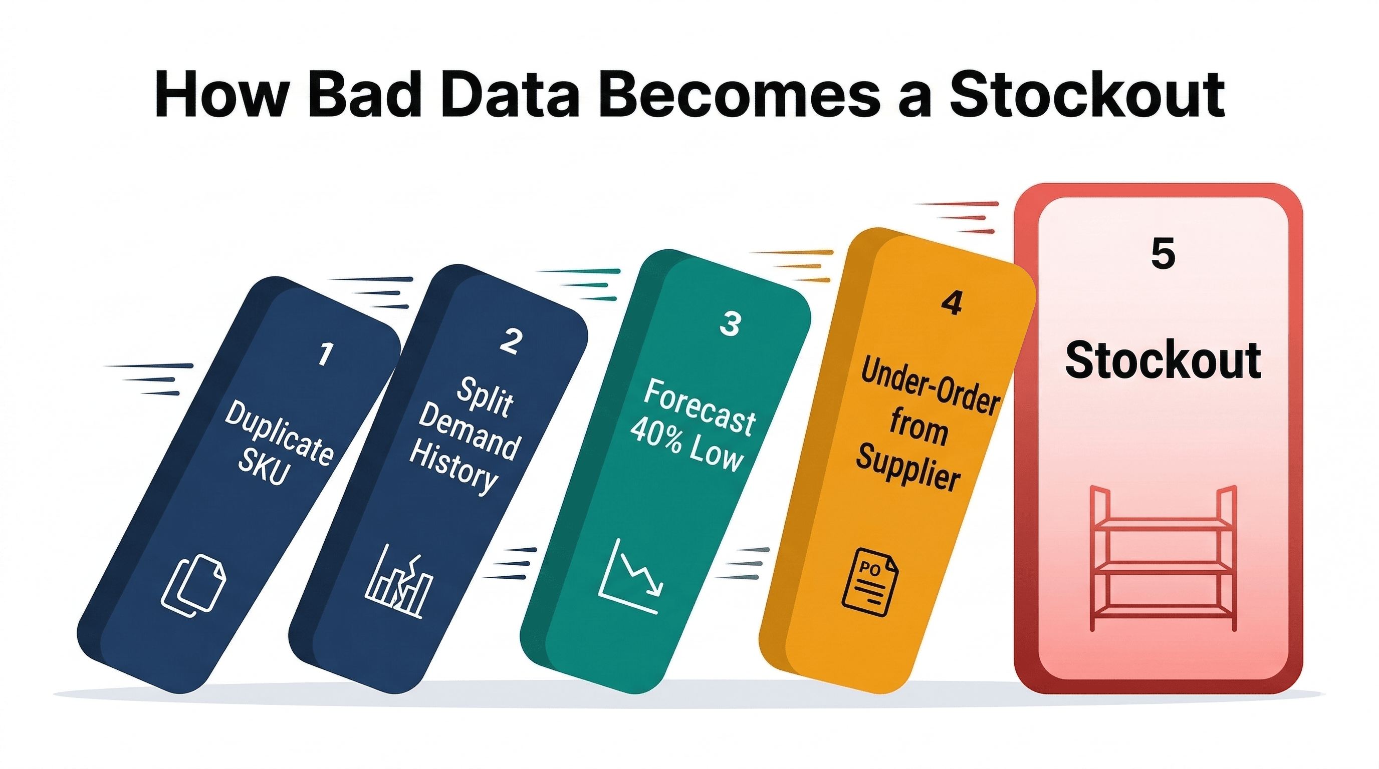
Your Inventory Data Is Wrong
How bad SKU data (duplicates, missing costs, unmatched listings, missing demand) breaks inventory forecasting and costs real money.
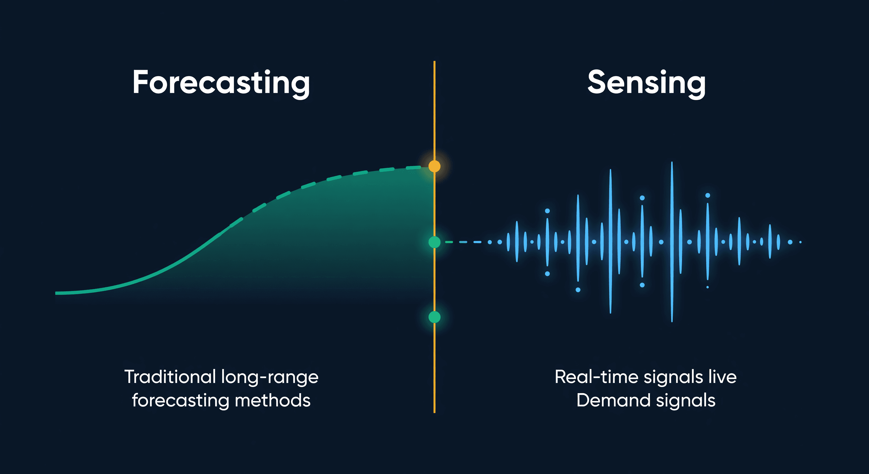
Demand Sensing vs Forecasting for E-commerce
What demand sensing actually is, how it differs from forecasting, why most e-commerce sellers only need one of them, and the practical middle ground.
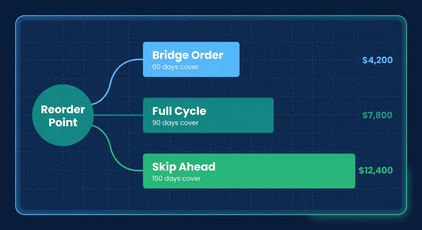
Three Ways to Place the Same Order
Bridge, Full Cycle, and Skip Ahead ordering strategies compared with worked cost numbers. When each one wins and how to pick.
